Open the “black box” of efficiency evaluation. Replacing rigid one-to-one price equality with conservation of the virtual value of intermediates yields a naturally unique decomposition of system efficiency and restores every stage efficiency to its true technical efficiency under its own production possibility set (PPS).
E* = E⁽¹⁾* × E⁽²⁾*
Overall system efficiency = the product of the two unique stage efficiencies
Conventional DEA treats each decision-making unit (DMU) as a “black box” whose internal structure is invisible. Two-stage and generalized network DEA opened that box and captured the flow of intermediates inside the system, yet they have long been constrained by multiple optimal solutions of the multiplier model.
1
Non-unique decomposition
Although overall system efficiency is uniquely determined, the multiplier model often has multiple optimal solutions, so the stage efficiency values obtained from the decomposition are not unique and the algebraic mapping between system and node efficiencies is unstable.
2
Distorted stage efficiencies
Stage efficiencies decomposed under rigid synergy need not be the true technical efficiencies of the stages under their own PPS: E⁽¹⁾ ≤ E⁽¹⁾*, E⁽²⁾ ≤ E⁽²⁾*.
3
Artificially “locked” results
Previous studies mostly relied on secondary objectives, subjective preference weights, or leader–follower game models to forcibly pin down a decomposition, introducing extra assumptions and subjectivity.
An unstable decomposition also obstructs further analysis of node efficiency values — for example, TFP index (Malmquist / HMB) analysis at the node level and intertemporal comparisons.
02 · THE BREAKTHROUGH
Flexible synergy: conservation of the virtual value of intermediates
The MaxDEA team abandons the strong exogenous constraint that the price of every intermediate must be equal one-to-one, and instead requires only that the total value of all intermediates of the evaluated DMU be equal as they flow within the system. This single core change simultaneously delivers a unique decomposition of system efficiency and keeps the decomposed stage efficiencies consistent with the stand-alone technical efficiencies of the stages.
Aspect
Rigid Synergy
Flexible SynergyTHE MAXDEA MODEL
Multiplier model
One-to-one price equality w⁽¹⁾ = w⁽²⁾ Imposes a unified cross-stage “exogenous market price” on intermediate products
Equal total value w⁽¹⁾·z0 = w⁽²⁾·z0 Intermediate shadow prices are determined within the system by the classical DEA optimization principle
Envelopment model
Each intermediate scales freely and independently; radial and non-radial adjustment are mixed and projections deviate from the classical technology improvement path
Radial scaling of intermediates Z·λ⁽¹⁾ ≥ z0·τ ≥ Z·λ⁽²⁾ Fully preserves the classical radial proportional improvement path
Decomposition result
Stage efficiencies are distorted by the rigid constraint; the decomposition is not unique
Unique system-efficiency decomposition; stage efficiencies equal the technical efficiencies under each stage’s own PPS
Note: when the network contains only one intermediate, the two synergy mechanisms are equivalent (w⁽¹⁾·z0 = w⁽²⁾·z0 ⟺ w⁽¹⁾ = w⁽²⁾).
Shadow prices & production function theory
Stage 1 and Stage 2 embody different production technologies, so the marginal rates of substitution (MRS) of the intermediates differ. Forcing shadow prices to be equal one-to-one means fitting two independent convex frontiers with a single linear tangent plane, which inevitably distorts stage efficiencies. Flexible synergy grants w⁽¹⁾ and w⁽²⁾ independent degrees of freedom so each precisely matches the normal vector of its own optimal frontier (its locally optimal shadow prices).
Weighted virtual input–output theory
Intermediates play a dual role: the virtual output of Stage 1 and the virtual input of Stage 2. Flexible synergy removes this over-constraint and requires only that the virtual aggregated value of the intermediates be equal at the junction — neither created out of nothing nor destroyed without reason. This matches the closed-loop, no-externality character of intermediate products while preserving each stage’s complete freedom to seek its optimal weights.
03 · WHY IT MATTERS
Four verifiable advantages
1
A unique equality
System efficiency and the two stage efficiencies naturally satisfy a unique equality, with no additional conditions; a rigorous upper- and lower-bound proof is given in the appendix.
E* = E⁽¹⁾* × E⁽²⁾*
2
True stage efficiencies
The decomposed stage efficiency is precisely the technical efficiency of that stage under its own PPS, ready for node-level TFP index analysis.
E⁽ᵗ⁾ = E⁽ᵗ⁾*
3
Classical improvement path
It fully adopts the classical radial proportional technology improvement path, completely preserving the economic meaning of the classical dual multiplier model.
Z·λ⁽¹⁾ ≥ z0·τ ≥ Z·λ⁽²⁾
4
No subjective settings
No secondary objectives, preference weights or leader–follower games: the result is uniquely determined by the model itself and reproducible.
No artificial “lock-in”
04 · SERIAL EFFECT
Why system efficiency decomposition in two-stage network models must take the product form
The multiplicative structure avoids excessive substitution compensation, in which a highly efficient stage would overly compensate for an inefficient one. “Neither stage may fall behind” is inherent to a serial system: the inefficiency of any sub-stage drags down overall system efficiency multiplicatively.
Example · Companies A and B make the same product from the same raw materials
Company
Stage 1 efficiency
Stage 2 efficiency
System efficiency
Company A (benchmark)
1.00
1.00
1.00
Company B
0.10
0.90
0.10 × 0.90 = 0.09
0.09Product form · the correct serial effect
0.5Arithmetic mean · clearly overstated
In Stage 1, company B uses 100 units of raw materials to produce only 10 units of intermediates (efficiency 0.1 relative to A); in Stage 2 it uses those 10 units to produce 9 units of final product (efficiency 0.9 relative to A). The product form correctly captures this serial-chain effect: overall efficiency is 0.09, not the 0.5 given by the arithmetic average.
05 · MODEL FAMILY
A complete family, from two stages to arbitrary topologies
9.1 · CRS
Two-stage network DEA (constant returns to scale)
Building on the multiplicative efficiency decomposition framework initiated by Kao & Hwang (2008) and Liang, Cook & Zhu (2008), the model is rebuilt on conservation of the virtual value of intermediates. The Charnes-Cooper transformation yields a linear program, and the appendix gives a rigorous proof of E* = E⁽¹⁾* × E⁽²⁾*.
Multiplier and dual envelopment models
Input-oriented / output-oriented
Unique decomposition equal to the product of stand-alone efficiencies
9.2 · VRS
Two-stage network DEA (variable returns to scale)
With the returns-to-scale constant u0⁽ᵗ⁾, complete input-oriented (intercept assigned to the output side) and output-oriented (intercept assigned to the input side) models are given; the efficiency decomposition again satisfies the unique multiplicative relationship.
Input-oriented: intercept on the output side
Output-oriented: intercept on the input side
Same multiplicative decomposition as the CRS model
9.3 · GENERAL
Generalized network DEA
Covers multiple nodes with serial, parallel and arbitrary topologies. The objective is a sum of fractions — a nonlinear program that must also allow proportional scaling of node weights — so it cannot be linearized by the Charnes-Cooper transformation and is solved by the Dinkelbach parametric approach. Stand-alone node models are solved first for E⁽ᵗ⁾*, then D* determines whether synergy is lossless.
D* = 0: lossless synergy, node efficiencies unique and equal to stand-alone values
D* < 0: lossy synergy, node efficiency values are not unique
Power-product system efficiency E* = Π(E⁽ᵗ⁾*)^ω⁽ᵗ⁾
Figure 2 Node weights in a mixed serial–parallel network: start with weight 1 for serial nodes, then halve the weights of nodes inside each parallel branch. ω⁽ᵗ⁾=1 gives the product (serial); Σω⁽ᵗ⁾=1 gives the geometric mean (parallel).
Node weights ω⁽ᵗ⁾ determine how system efficiency is aggregated The product form applies to serial structures and the geometric mean to parallel structures. In empirical studies, final weights can also reflect the importance of each node to the system.
9.4 · FDEF
Generalized network DEA based on full-dimensional efficient facets
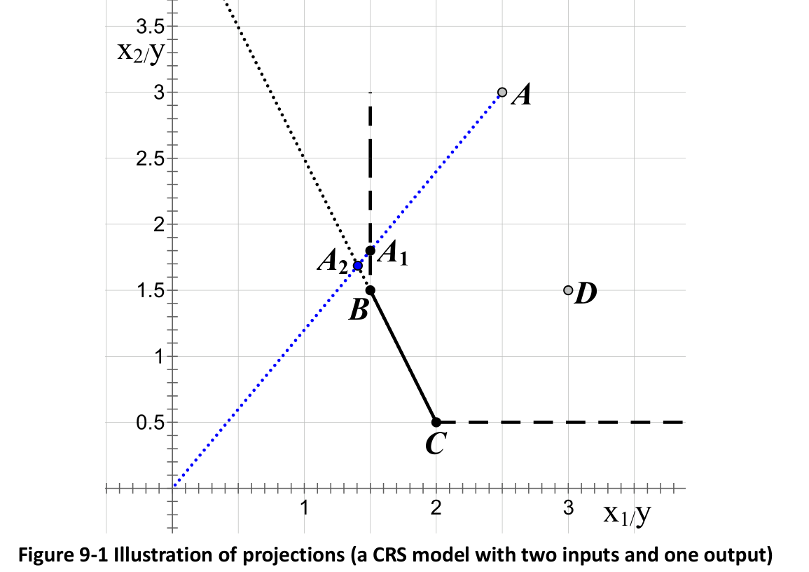
Weights are restricted to the set of FDEF hyperplanes of each stage. Because all weights are strictly greater than zero, input, output and intermediate slacks are completely eliminated and the projected intermediate values on the two sides coincide exactly. A single simple sufficient condition achieves lossless synergy and unique decomposition: the network contains a node that only produces intermediates without consuming any, and a node that only consumes intermediates without producing any.
Eliminates zero weights and all slacks
Finite, non-zero and determinate marginal rates of substitution
The two-stage model satisfies the condition naturally
Figure 9-1 Illustration of projections (a CRS model with two inputs and one output): A₂, the radial projection based on the FDEF affine hull, is more reasonable than C, the projection given by non-radial models.
06 · IN MAXDEA X
Ready to use in MaxDEA X
All of these models are integrated in MaxDEA X 13.0 and can be freely combined with every panel data model. Four setup steps, results delivered directly.
1
Define the data
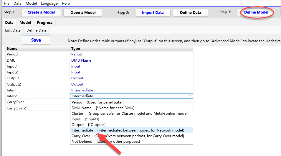
Set the variables flowing between nodes to type Intermediate; define the rest as inputs, outputs, DMU names and so on.
2
Set general options
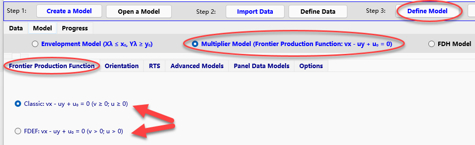
Choose the production function type (classical frontier production function or FDEF affine-hull frontier production function), model orientation and returns to scale.
3
Select the network model
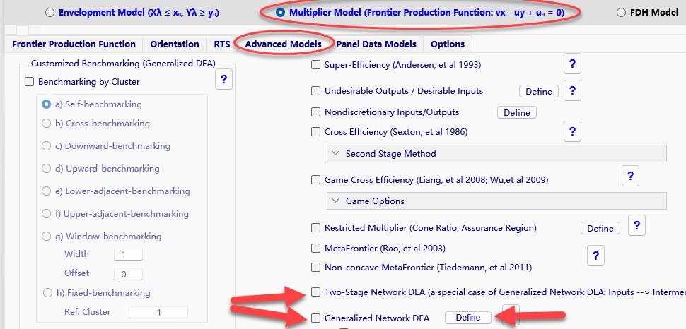
Under “Advanced Models”, select “Two-Stage Network DEA” or “Generalized Network DEA”. Network DEA combines with all panel data models: Malmquist TFP index, HMB TFP index, window DEA and Carry-Over DEA.
4
Define the network structure
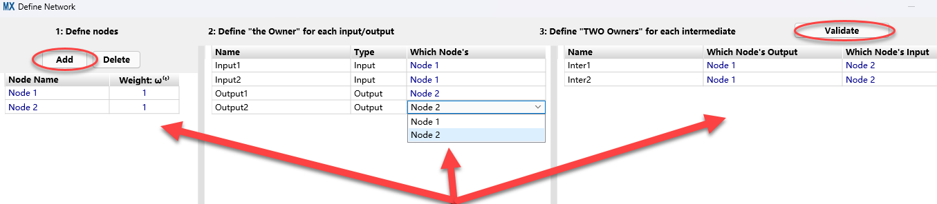
For generalized network DEA, define the nodes, the owner of each input/output and the “two owners” of each intermediate, then Validate. The default node weight is ω⁽ᵗ⁾=1 (product); set Σω⁽ᵗ⁾=1 for a geometric mean.
Click a screenshot to enlarge
Results
Overall system efficiency; weights and projected values (targets) of inputs, outputs and intermediates; node efficiency values; node benchmarks and their coefficients (Lambda). VRS models also report the returns-to-scale constant u₀⁽ᵗ⁾, and generalized network models report D*, used to determine whether the node efficiency values are unique.
07 · CITE & RESOURCES
Cite & resources
English citation
MaxDEA Team. (2026-10-26). Innovative Two-Stage and Generalized Network DEA. MaxDEA. https://maxdea.com/2026/202609.pdf.
All model definitions, dual derivations, the proof of multiplicative efficiency decomposition for CRS two-stage network DEA, notation and data conventions, a software walkthrough and references — in both Chinese and English.
Kao, C., & Hwang, S.-N. (2008). Efficiency decomposition in two-stage data envelopment analysis. European Journal of Operational Research, 185(1), 418–429.
Liang, L., Cook, W. D., & Zhu, J. (2008). DEA models for two-stage processes: Game approach and efficiency decomposition. Naval Research Logistics, 55(7), 643–653.
Olesen, O. B., & Petersen, N. C. (1996). Indicators of ill-conditioned data sets and model misspecification in DEA. Management Science, 42(2), 205–219.
Olesen, O. B., & Petersen, N. C. (2003). Identification and use of efficient faces and facets in DEA. Journal of Productivity Analysis, 20(3), 323–360.
Olyaie, M. D., Roshdi, I., Jahanshahloo, G., & Asgharian, M. (2014). Characterizing and finding full dimensional efficient facets in DEA. JORS, 65(9), 1453–1464.
Make network efficiency decomposition unique and true again
MaxDEA X 13.0 fully supports the innovative two-stage network DEA, generalized network DEA and FDEF-based generalized network DEA, running natively on Windows, macOS and Linux.